pimeta Package

pimeta Package (CRAN)
メタアナリシスの予測区間 (Higgins et al., 2009; Partlett & Riley, 2017; Nagashima et al., 2019) を実装した R パッケージです。

CRAN Task View の MetaAnalysis に登録されています (2018/04/20現在)

メタアナリシスにおける予測区間の解析スクリプト例

pimeta パッケージでは、比較的少ない量のスクリプトで解析が実行できるようになっています。
以下は、連続アウトカムデータと二値アウトカムデータから予測区間を計算し、フォレストプロットを作成するスクリプト例です。
予測区間を計算する pima 関数に各試験の平均値 "y" と標準誤差 "se" を指定して実行します (詳細は関数のヘルプファイルをご参照ください)。二値アウトカムデータは、"convert_bin" 関数を使って対数オッズ比 "logOR"、対数リスク比 "logRR"、リスク差 "RD"、に変換できます、"m1", "m2" は各群内のイベント数で "n1", "n2" は各群内の総例数です (詳細は関数のヘルプファイルをご参照ください)。


  ### Install package if necessary
  if (!require("pimeta")) {install.packages("pimeta"); require("pimeta")}

  ### The 'pimeta' package
  sbp <- data.frame(
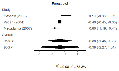
    y = c(0.10, -0.40, -0.80),
    sigmak = c(0.21939179, 0.02551067, 0.19898325),
    label = c("Cashew (2003)", "Pecan (2004)",
              "Macadamia (2007)")
  )
  print(sbp)
  piboot <- pima(sbp$y, sbp$sigmak, seed = 3141592, parallel = 4)
  print(piboot)

  png("forestplot.png", width = 500, height = 300, family = "Arial")
  plot(piboot, digits = 2, base_size = 18, studylabel = sbp$label)
  dev.off()

  ### Random-effects meta-analysis with binary outcome
  m1 <- c(15,12,29,42,14,44,14,29,10,17,38,19,21)
  n1 <- c(16,16,34,56,22,54,17,58,14,26,44,29,38)
  m2 <- c( 9, 1,18,31, 6,17, 7,23, 3, 6,12,22,19)
  n2 <- c(16,16,34,56,22,55,15,58,15,27,45,30,38)
  dat <- convert_bin(m1, n1, m2, n2, type = "logOR")
  print(dat)
  pibin <- pima(dat$y, dat$se, seed = 2236067, parallel = 4)
  print(pibin, trans = "exp")
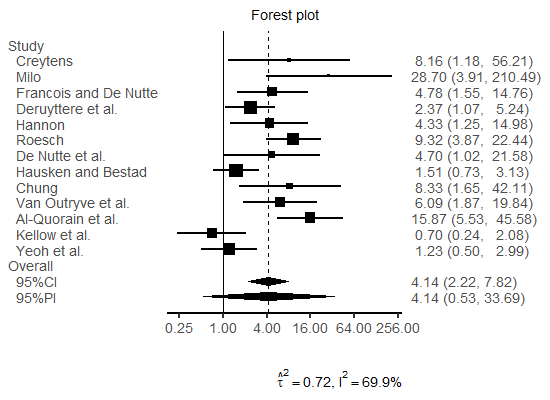
  binlabel <- c(
    "Creytens", "Milo", "Francois and De Nutte", "Deruyttere et al.",
    "Hannon", "Roesch", "De Nutte et al.", "Hausken and Bestad",
    "Chung", "Van Outryve et al.", "Al-Quorain et al.", "Kellow et al.",
    "Yeoh et al.")
  png("forestplot_bin.png", width = 550, height = 400, family = "Arial")
  plot(pibin, digits = 2, base_size = 18, studylabel = binlabel, trans = "exp")
  dev.off()

実行結果の抜粋です。


  > print(sbp)
        y     sigmak            label
  1  0.1 0.21939179    Cashew (2003)
  2 -0.4 0.02551067     Pecan (2004)
  3 -0.8 0.19898325 Macadamia (2007)
  > piboot <- pima(sbp$y, sbp$sigmak, seed = 3141592, parallel = 4)
  > print(piboot)

  Prediction & Confidence Intervals for Random-Effects Meta-Analysis

  A parametric bootstrap prediction and confidence intervals
    Heterogeneity variance: DerSimonian-Laird
    Variance for average treatment effect: Hartung (Hartung-Knapp)

  No. of studies: 3

  Average treatment effect [95% prediction interval]:
    -0.3804 [-2.2704, 1.5108]
    d.f.: 2

  Average treatment effect [95% confidence interval]:
    -0.3804 [-1.4498, 0.6573]
    d.f.: 2

  Heterogeneity measure
    tau-squared: 0.0803
    I-squared:  78.3%

forest plot


  > ### Random-effects meta-analysis with binary outcome
  > m1 <- c(15,12,29,42,14,44,14,29,10,17,38,19,21)
  > n1 <- c(16,16,34,56,22,54,17,58,14,26,44,29,38)
  > m2 <- c( 9, 1,18,31, 6,17, 7,23, 3, 6,12,22,19)
  > n2 <- c(16,16,34,56,22,55,15,58,15,27,45,30,38)
  > dat <- convert_bin(m1, n1, m2, n2, type = "logOR")
  > print(dat)
              y        se
  1   2.0989861 0.9847737
  2   3.3570262 1.0165653
  3   1.5652318 0.5747840
  4   0.8640463 0.4042977
  5   1.4656407 0.6332968
  6   2.2325713 0.4481371
  7   1.5465488 0.7782417
  8   0.4125323 0.3721812
  9   2.1202635 0.8265438
  10  1.8071598 0.6022988
  11  2.7646729 0.5382109
  12 -0.3544099 0.5555283
  13  0.2058521 0.4541130
  > pibin <- pima(dat$y, dat$se, seed = 2236067, parallel = 4)
  > print(pibin, trans = "exp")

  Prediction & Confidence Intervals for Random-Effects Meta-Analysis

  A parametric bootstrap prediction and confidence intervals
    Heterogeneity variance: DerSimonian-Laird
    Variance for average treatment effect: Hartung (Hartung-Knapp)

  No. of studies: 13

  Average treatment effect [95% prediction interval]:
    4.1408 [0.5335, 33.6922]
    d.f.: 12
    Scale: exponential transformed

  Average treatment effect [95% confidence interval]:
    4.1408 [2.2237, 7.8202]
    d.f.: 12
    Scale: exponential transformed

  Heterogeneity measure
    tau-squared: 0.7176
    I-squared:  69.9%

forest plot

データを csv ファイル等から読み込んで実行することもできます。
上記の連続アウトカムデータを csvファイルに入力し、これを読み込んで実行するスクリプトの例を示します。


  sbp <- read.csv("sbp.csv")
  pima(sbp$y, sbp$sigmak, parallel = 4)

手法の解説記事

変量効果モデルによるメタアナリシスの予測区間

アップデート情報

2019/09/24 1.1.3 機能追加 (対数オッズ比・対数リスク比の指数変換表示 [printおよびplotにtrans = "exp"オプションを追加]; Thanks to Dr. Morio Aihara)
2019/03/11 1.1.2 機能追加 (フォレストプロット、予測区間 [Bootstrap法のマルチスレッド化、Kenward–Rogerのアプローチ]、信頼区間 [11種類の手法を追加]、$\hat{\tau}^2$の点推定 [12種類の手法を追加]、$\hat{\tau}^2$の区間推定 [最尤法とREMLを追加]、二値アウトカムデータ用の変換関数の追加 [対数オッズ比、対数リスク比、リスク差])
2018/09/15 1.1.1 ドキュメントの修正。
2018/09/14 1.1.0 パッケージ内部構造の最適化。Vignette ファイルの作成。
2018/05/11 1.0.1 文献情報の修正
2018/04/05 1.0.0 公開版をCRANにリリース; 2018/04/19 に CRAN Task View の MetaAnalysis に登録されました。

引用文献

Higgins JPT, Thompson SG, Spiegelhalter DJ. A re-evaluation of random-effects meta-analysis. Journal of the Royal Statistical Society: Series A (Statistics in Society) 2009; 172(1): 137–159. doi:10.1111/j.1467-985X.2008.00552.x.
Partlett C, Riley RD. Random effects meta-analysis: Coverage performance of 95% confidence and prediction intervals following REML estimation. Statistics in Medicine 2017; 36(2): 301–317. doi:10.1002/sim.7140.
Nagashima K, Noma H, Furukawa TA. Prediction intervals for random-effects meta-analysis: a confidence distribution approach. Statistical Methods in Medical Research 2019; 28(6): 1689–1702. doi: 10.1177/0962280218773520. [arXiv:1804.01054]

履歴

2019/09/24 v1.1.3の情報を追加しました。
2019/09/10 日本語の解析用スクリプトの解説を書きました (Thanks to Dr. Morio Aihara)。
2018/06/12 解説記事を別に作成して整理しました
2018/05/10 文献情報のアップデート
2018/04/10 公開