kmdata その他のコンテンツ
サンプルプログラム
以下で示すサンプルプログラムでは、まず初期設定、マクロとデータの読み込みを行います。
generator ではサンプルデータを自動生成することができます。以下で示している事例についても簡単に生成できます。
example.zip (download)
  proc datasets lib = work kill; run;
  option linesize = 200 pagesize = 5000 mprint;
  dm 'log; clear; output; clear;';

  /* setting path */
  %let execpath = " ";
  %let Path = " ";
  %macro setexecpath;
    %let execpath = %sysfunc(getoption(sysin));
    %if %length(&execpath) = 0 %then
      %let execpath = %sysget(sas_execfilepath);
    data _null_;
      do i = length("&execpath") to 1 by -1;
        if substr("&execpath", i, 1) = "\" then do;
          call symput("Path", substr("&execpath", 1, i));
          stop;
        end;
      end;
    run;
  %mend setexecpath;
  %setexecpath;
  libname Out "&Path";

  /* set global macro variables for censor extension */
  %global color1 color2 color3 scolor1 scolor2 scolor3;
  %include "&Path.kmdata_v221.sas";
  %let filetype = bmp;

  data D1;
    length GroupC $20.;
    call streaminit(32789238);
    tc = 12;  /* withdrawal time */
    h1 = 0.100;  n1 = 50; /* h1: hazard of group 1 */
    h2 = 0.075;  n2 = 50; /* h2: hazard of group 2 */
    h2 = 0.050;  n3 = 50; /* h2: hazard of group 3 */
    /* E(T)=1/h */
    array h[*] h1-h2; array n[*] n1-n3;
    do Group = 1 to 3;
      do i = 1 to n[group];
        T = rand('exponential') / h[group]; Censor = 0;
        if T > tc then do; T = tc; Censor = 1; end;
        if rand('Uniform') > 0.9 then do; Censor = 1; end;
  /* lost to follow-up (random) */
        if Group = 1 then do; GroupC = '1: high-risk'; GroupC2 = 'high-risk'; end;
        if Group = 2 then do; GroupC = '2: middle-risk'; GroupC2 = 'middle-risk'; end;
        if Group = 3 then do; GroupC = '3: low-risk'; GroupC2 = 'low-risk'; end;
        output;
      end;
    end;
    label T = "Months after entry";
    keep T Censor Group GroupC GroupC2;
  run;

  /*****************************************************************/
  /* Color pattern */
  %let color1  = cx445694;
  %let color2  = cxA23A2E;
  %let color3  = cx01665E;

  %let scolor1 = cxD4D9E8;
  %let scolor2 = cxF1CECE;
  %let scolor3 = cxD1E4E3;
上では、色の設定を 3 色しか行っていませんので、4 層以上のグラフを出力したい場合、または色を変えたい場合はこの部分を修正してください (generator では 4 色分設定しています)。
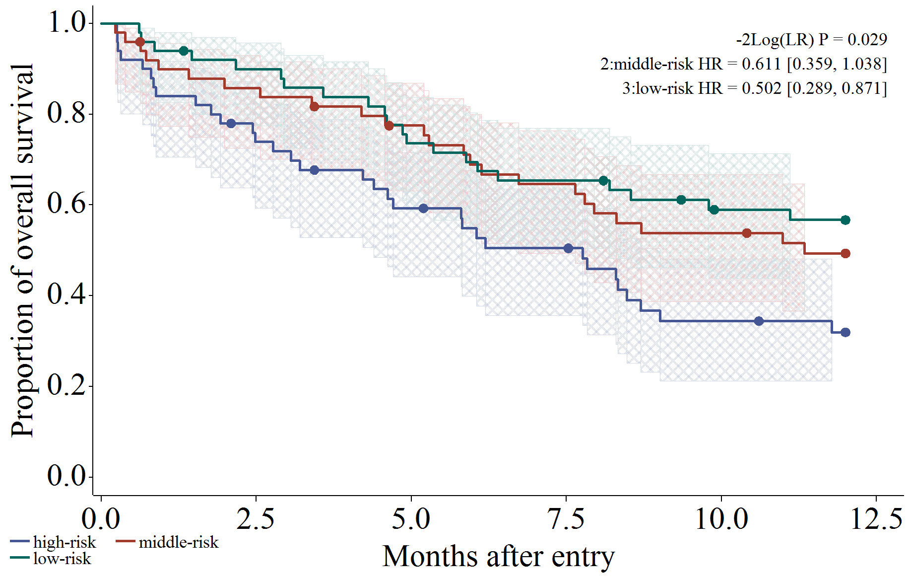
以下では実行例が続きます。信頼区間 (メッシュ)、打ち切り (ヒゲ)、リスク集合の大きさ (表示)、Log-rank 検定、ハザード比を出力するように設定した場合です。
  /*****************************************************************/
  /* CI: fill, Censor: needle, Atrisk: show, Logrank test, Hazardratio */
  %km_data(
    D1, T, GroupC, Censor, 1,
    out = graph, anno = anno,

    CI = 1,
    censEXT = 1,

    Size = 2,
    atrisk = 1, atriskorder = 0 to 12.5 by 2.5, Step = 5,
    Label = "No. at risk (1st entry: high, 2nd: middle, 3rd: low)",
    Test = 1, TestX = 98, TestY = 97, Type = logrank,
    HR = 1, HRX = 98, HRY = 92
  );
  goptions reset = all;
  goptions vsize = 12 in hsize = 19 in htitle = 3.5 htext = 3.5;
  options linesize = 98 pagesize = 200;
  filename grafout "&Path.example1.&filetype.";
  goptions device = &filetype. gsfname = grafout gsfmode = replace;
  goptions ftext = "Times New Roman";
  proc gplot data = Graph;
    plot (Sv1 Sv2 Sv3) * T /
        anno = anno /* autovref cautovref = cxE9DECA */
        overlay skipmiss noframe legend = legend1
        haxis = axis1 vaxis = axis2;
    axis1 label = ('Months after entry') major=(w=2 height=0.7) w=2 minor = none
      order = (0 to 12.5 by 2.5) offset = (2, 7);
    axis2 label = (a=90 'Proportion of overall survival') major=(w=2 height=1)
      w=2 minor = none offset = (2, 2) order = (0 to 1 by 0.2);
    legend1 label = none position = (inside) mode = share across = 2
      origin = (2, 1) value = (h = 2 "high-risk" "middle-risk" "low-risk");
    symbol1 i = steplj c="&color1." w = 5;
    symbol2 i = steplj c="&color2." w = 5;
    symbol3 i = steplj c="&color3." w = 5;
  run; quit;

信頼区間 (メッシュ)、打ち切り (点を Gplot で描画)、Log-rank 検定、ハザード比を出力するように設定した場合です。
legend statment で order オプションを利用するために、データセットを編集しています。
  /*****************************************************************/
  /* CI: fill, Censor: dot, Atrisk: none, Likelihood ratio test, Hazardratio */
  %km_data(
    D1, T, GroupC, Censor, 1,
    out = graph, anno = anno,

    CI = 1,
    censEXT = 0,

    Size = 2, Step = 5,
    atrisk = 0,
    Test = 1,  TestX = 98, TestY = 97, Type = likelihoodratio,
    HR = 1, HRX = 98, HRY = 92
  );
  goptions reset = all;
  goptions vsize = 12 in hsize = 19 in htitle = 3.5 htext = 3.5;
  options linesize = 98 pagesize = 200;
  filename grafout "&Path.example2.&filetype.";
  goptions device = &filetype. gsfname = grafout gsfmode = replace;
  goptions ftext = "Times New Roman";
  data Graph;
    length vname $10.;
    set Graph;
    var=Sv1; vname='Sv1'; output;
    var=Sv2; vname='Sv2'; output;
    var=Sv3; vname='Sv3'; output;
    var=CSDF1; vname='zCSDF1'; output;
    var=CSDF2; vname='zCSDF2'; output;
    var=CSDF3; vname='zCSDF3'; output;
  proc sort data = Graph; by vname T;
  proc gplot data = Graph;
    plot var * T = vname/
        anno = anno /* autovref cautovref = cxE9DECA */
        skipmiss noframe legend = legend1
        haxis = axis1 vaxis = axis2;
    axis1 label = ('Months after entry') major=(w=2 height=0.7) w=2 minor = none
      order = (0 to 12.5 by 2.5) offset = (2, 7);
    axis2 label = (a=90 'Proportion of overall survival') major=(w=2 height=1)
      w=2 minor = none offset = (2, 2) order = (0 to 1 by 0.2);
    legend1 label = none position = (inside) mode = share across = 2
      origin = (2, 1) value = (h = 2 "high-risk" "middle-risk" "low-risk")
      order = ("Sv1" "Sv2" "Sv3");
    symbol1 i = steplj c="&color1." w = 5;
    symbol2 i = steplj c="&color2." w = 5;
    symbol3 i = steplj c="&color3." w = 5;
    symbol4 i = none c="&color1." h = 2 v = dot;
    symbol5 i = none c="&color2." h = 2 v = dot;
    symbol6 i = none c="&color3." h = 2 v = dot;
  run; quit;
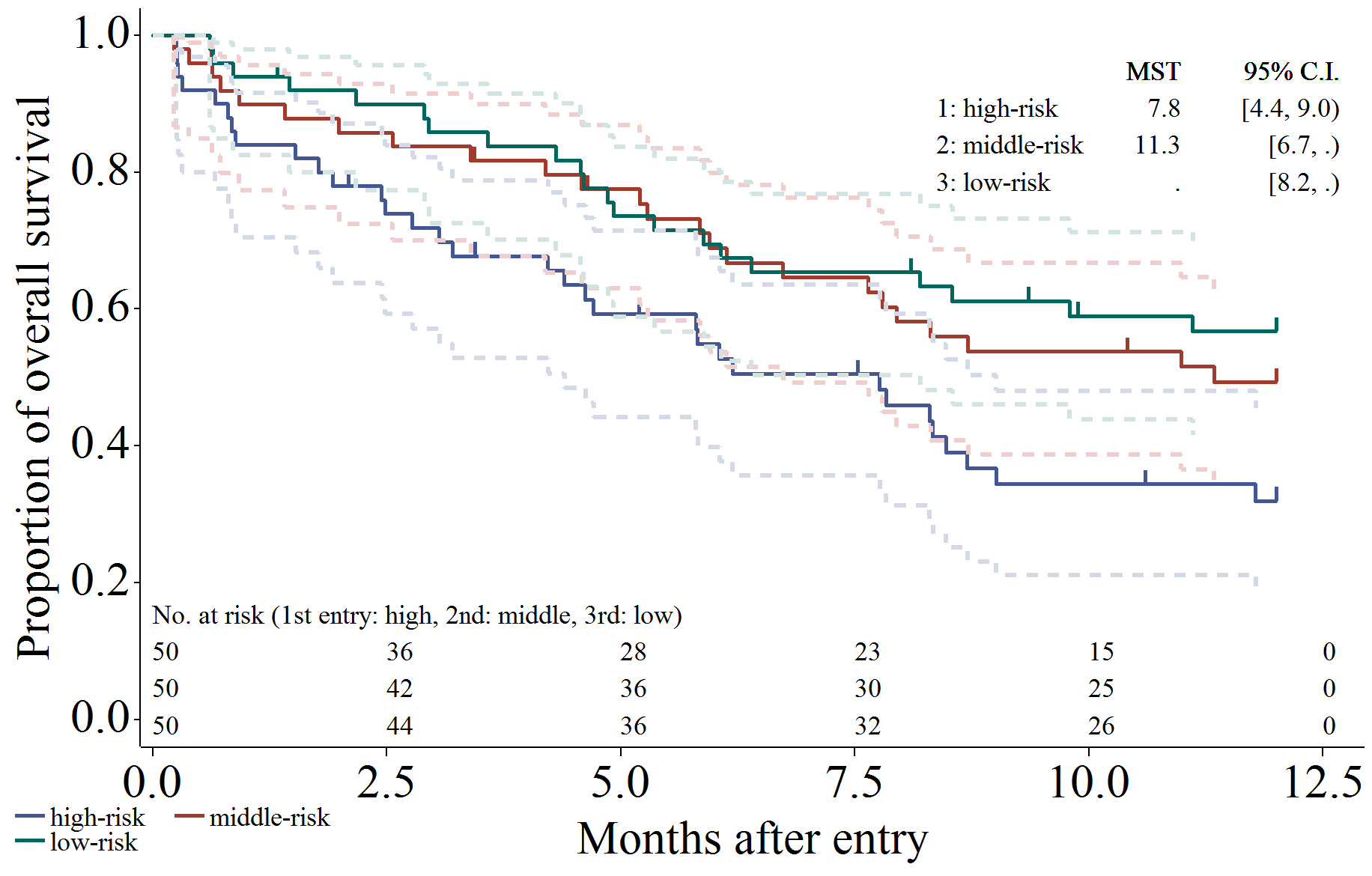
信頼区間 (線を Gplot で描画)、打ち切り (ヒゲ)、リスク集合の大きさ (表示)、生存期間中央値と95%信頼区間を出力するように設定した場合です。
こちらも legend statment で order オプションを利用するために、データセットを編集しています。
  /*****************************************************************/
  /* CI: line, Censor: needle, Atrisk: show, MST */
  %km_data(
    D1, T, GroupC, Censor, 1,
    out = graph, anno = anno,

    CI = 0,
    censEXT = 1,

    Size = 2, Step = 5,
    atrisk = 1, atriskorder = 0 to 12.5 by 2.5,
    Label = "No. at risk (1st entry: high, 2nd: middle, 3rd: low)",
    Test = 0,
    HR = 0,
    MST = 1, MlabX = 65, MmedX = 85, MciX = 98, MSTY = 97
  );
  goptions reset = all;
  goptions vsize = 12 in hsize = 19 in htitle = 3.5 htext = 3.5;
  options linesize = 98 pagesize = 200;
  filename grafout "&Path.example3.&filetype.";
  goptions device = &filetype. gsfname = grafout gsfmode = replace;
  goptions ftext = "Times New Roman";
  data Graph;
    length vname $10.;
    set Graph;
    var=Sv1; vname='Sv1'; output;
    var=Sv2; vname='Sv2'; output;
    var=Sv3; vname='Sv3'; output;
    var=SL1; vname='zSL1'; output;
    var=SL2; vname='zSL2'; output;
    var=SL3; vname='zSL3'; output;
    var=SU1; vname='zSU1'; output;
    var=SU2; vname='zSU2'; output;
    var=SU3; vname='zSU3'; output;
  proc sort data = Graph; by vname T;
  proc gplot data = Graph;
    plot var * T = vname/
        anno = anno /* autovref cautovref = cxE9DECA */
        skipmiss noframe legend = legend1
        haxis = axis1 vaxis = axis2;
    axis1 label = ('Months after entry') major=(w=2 height=0.7) w=2 minor = none
      order = (0 to 12.5 by 2.5) offset = (2, 7);
    axis2 label = (a=90 'Proportion of overall survival') major=(w=2 height=1)
      w=2 minor = none offset = (2, 2) order = (0 to 1 by 0.2);
    legend1 label = none position = (inside) mode = share across = 2
      origin = (2, 1) value = (h = 2 "high-risk" "middle-risk" "low-risk")
      order = ("Sv1" "Sv2" "Sv3");
    symbol1 i = steplj c="&color1." w = 5;
    symbol2 i = steplj c="&color2." w = 5;
    symbol3 i = steplj c="&color3." w = 5;
    symbol4 i = steplj c="&scolor1." w = 5 l = 2;
    symbol5 i = steplj c="&scolor2." w = 5 l = 2;
    symbol6 i = steplj c="&scolor3." w = 5 l = 2;
    symbol7 i = steplj c="&scolor1." w = 5 l = 2;
    symbol8 i = steplj c="&scolor2." w = 5 l = 2;
    symbol9 i = steplj c="&scolor3." w = 5 l = 2;
  run; quit;
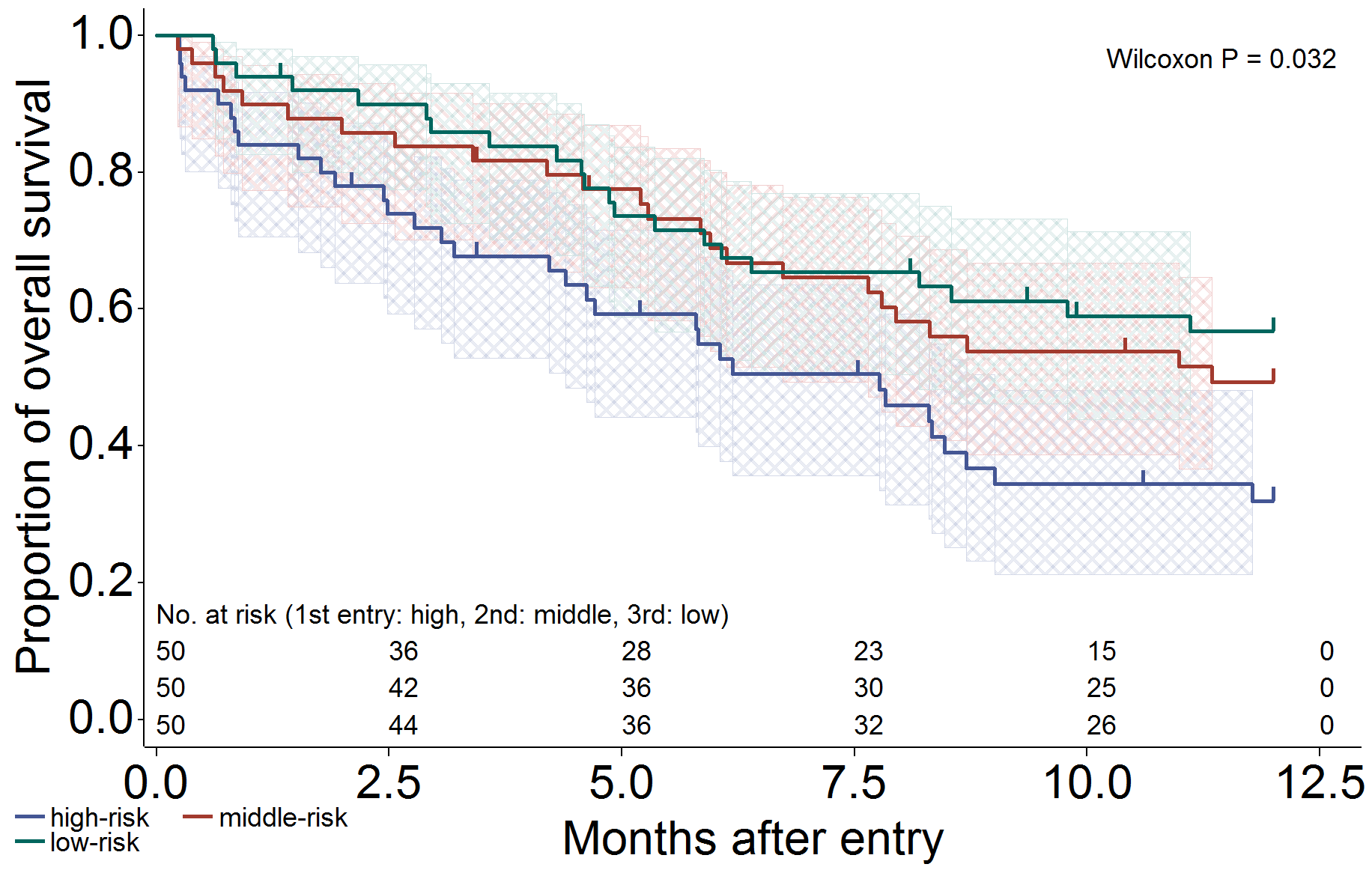
信頼区間 (メッシュ)、打ち切り (ヒゲ)、リスク集合の大きさ (表示)、一般化 Wilcoxon 検定を出力し、フォントを変更するように設定した場合です。
  /*****************************************************************/
  /* CI: fill, Censor: needle, Atrisk: show, generalized wilcoxon test */
  /* Font change!! */
  %km_data(
    D1, T, GroupC, Censor, 1,
    out = graph, anno = anno,

    CI = 1,
    censEXT = 1,

    Size = 2, Step = 5,
    afont = "'Arial'",
    atrisk = 1, atriskorder = 0 to 12.5 by 2.5,
    Label = "No. at risk (1st entry: high, 2nd: middle, 3rd: low)",
    Test = 1, TestX = 98, TestY = 97, Type = wilcoxon,
    HR = 0
  );
  goptions reset = all;
  goptions vsize = 12 in hsize = 19 in htitle = 3.5 htext = 3.5;
  options linesize = 98 pagesize = 200;
  filename grafout "&Path.example4.&filetype.";
  goptions device = &filetype. gsfname = grafout gsfmode = replace;
  goptions ftext = "Arial";
  proc gplot data = Graph;
    plot (Sv1 Sv2 Sv3) * T /
        anno = anno /* autovref cautovref = cxE9DECA */
        overlay skipmiss noframe legend = legend1
        haxis = axis1 vaxis = axis2;
    axis1 label = ('Months after entry') major=(w=2 height=0.7) w=2 minor = none
      order = (0 to 12.5 by 2.5) offset = (2, 7);
    axis2 label = (a=90 'Proportion of overall survival') major=(w=2 height=1)
      w=2 minor = none offset = (2, 2) order = (0 to 1 by 0.2);
    legend1 label = none position = (inside) mode = share across = 2
      origin = (2, 1) value = (h = 2 "high-risk" "middle-risk" "low-risk");
    symbol1 i = steplj c="&color1." w = 5;
    symbol2 i = steplj c="&color2." w = 5;
    symbol3 i = steplj c="&color3." w = 5;
  run; quit;
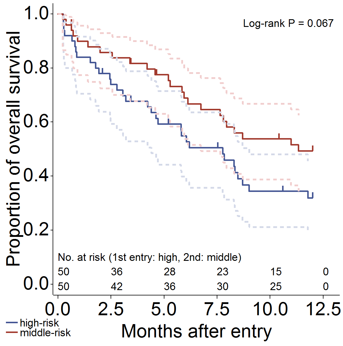
信頼区間 (線を Gplot で描画)、打ち切り (ヒゲ)、Log-rank 検定、リスク集合の大きさ (表示) を出力し、グラフのアスペクト比を変えた場合の設定例です。
  /*****************************************************************/
  /* CI: line, Censor: needle, Atrisk: show */
  /* aspect ratio "12:12" (for presentation), 2group */
  data D2; set D1; where Group in (1, 2);
  %km_data(
    D2, T, GroupC, Censor, 1,
    out = graph, anno = anno,

    CI = 0,
    censEXT = 1,

    Size = 2, Step = 5,
    afont = "'Arial'",
    atrisk = 1, atriskorder = 0 to 12.5 by 2.5,
    Label = "No. at risk (1st entry: high, 2nd: middle)",
    Test = 1,  TestX = 98, TestY = 97, Type = logrank,
    HR = 0
  );
  goptions reset = all;
  goptions vsize = 12 in hsize = 12 in htitle = 3.5 htext = 3.5;
  options linesize = 98 pagesize = 200;
  filename grafout "&Path.example5.&filetype.";
  goptions device = &filetype. gsfname = grafout gsfmode = replace;
  goptions ftext = "Arial";
  data Graph;
    length vname $10.;
    set Graph;
    var=Sv1; vname='Sv1'; output;
    var=Sv2; vname='Sv2'; output;
    var=SL1; vname='zSL1'; output;
    var=SL2; vname='zSL2'; output;
    var=SU1; vname='zSU1'; output;
    var=SU2; vname='zSU2'; output;
  proc sort data = Graph; by vname T;
  proc gplot data = Graph;
    plot var * T = vname/
        anno = anno /* autovref cautovref = cxE9DECA */
        skipmiss noframe legend = legend1
        haxis = axis1 vaxis = axis2;
    axis1 label = ('Months after entry') major=(w=2 height=0.7) w=2 minor = none
      order = (0 to 12.5 by 2.5) offset = (2, 7);
    axis2 label = (a=90 'Proportion of overall survival') major=(w=2 height=1)
      w=2 minor = none offset = (2, 2) order = (0 to 1 by 0.2);
    legend1 label = none position = (inside) mode = share across = 1
      origin = (2, 1) value = (h = 2 "high-risk" "middle-risk")
      order = ("Sv1" "Sv2");
    symbol1 i = steplj c="&color1." w = 5;
    symbol2 i = steplj c="&color2." w = 5;
    symbol3 i = steplj c="&scolor1." w = 5 l = 2;
    symbol4 i = steplj c="&scolor2." w = 5 l = 2;
    symbol5 i = steplj c="&scolor1." w = 5 l = 2;
    symbol6 i = steplj c="&scolor2." w = 5 l = 2;
  run; quit;
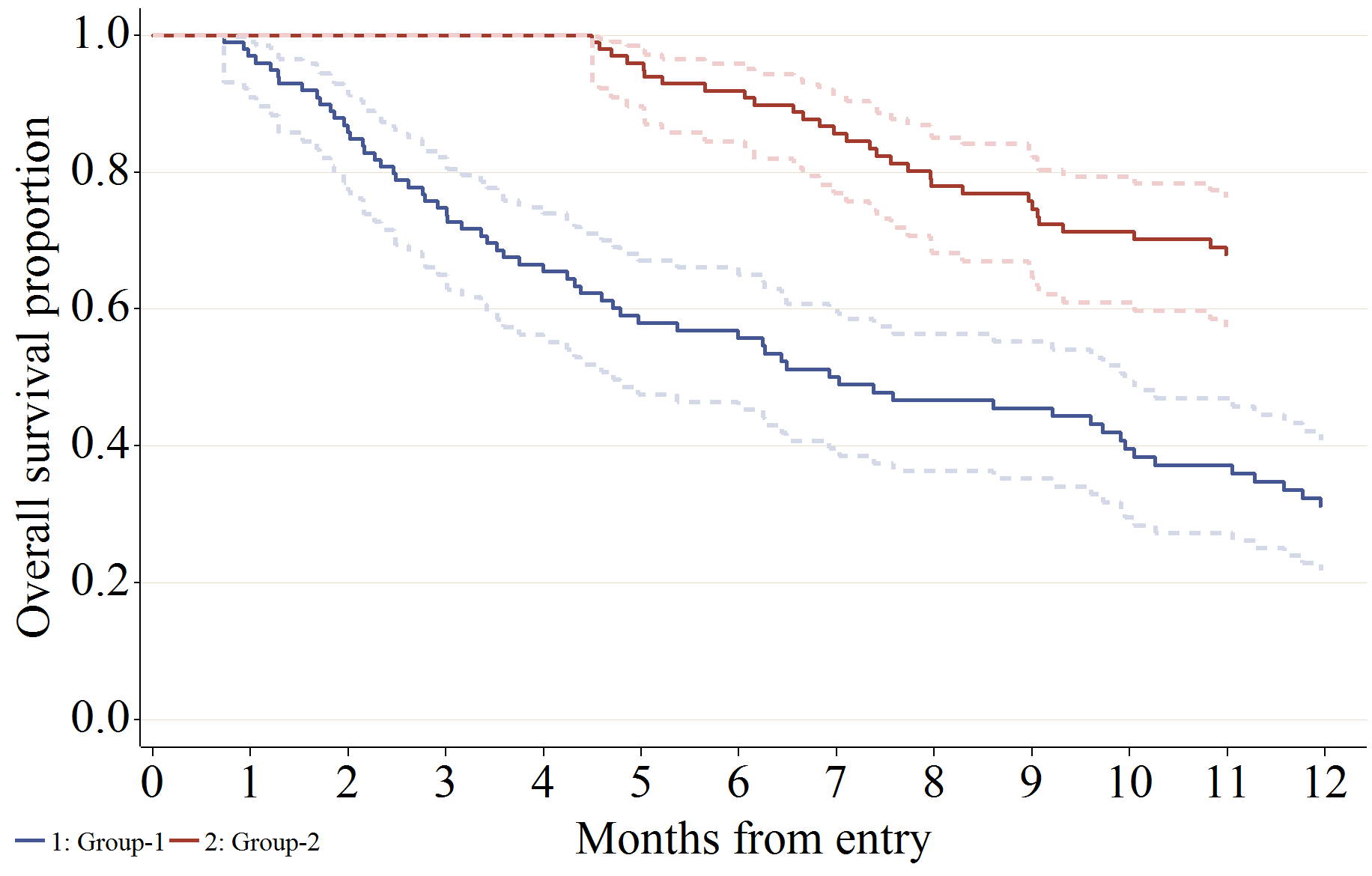
信頼区間 (線を Gplot で描画)、ベースラインの共変量の値で調整した生存関数の推定値を描画する場合の設定例です。
  /*****************************************************************/
  /* CI: line, baseline adjustment */
  data data;
    length strata $20.;
    call streaminit(8797348795);
    tc = 12;  /* time to termination */
    h1 = 0.15; n1 = 100;
    h1 = 0.07; n2 = 100;
    array h[*] h1-h1; array n[*] n1-n2;
    do group = 1 to 2;
      sex = rand("BERNOULLI", 0.1*group);
      baseline = group + rand("Normal");
      do i = 1 to n[group];
        time = baseline + sex + rand('exponential') / h[group]; censor = 0;
        /* termination */
        if time > tc then do; time = tc; censor = 1; end;
        /* random censoring */
        if rand('Uniform') > 0.9 then do; censor = 1; end;
        if group = 1 then do; strata = "1: Group-1"; end;
        if group = 2 then do; strata = "2: Group-2"; end;
        output;
      end;
    end;
    label time = "Months after entry";
    keep time censor group strata;
  run;
  proc summary data = data;
    class strata;
    var sex;
    output out = Cov00s mean = Sex;
  proc summary data = data;
    class strata;
    var baseline;
    output out = Cov00b mean = Baseline;
  data COV00;
    merge Cov00s Cov00b;
    by strata;
    where strata = "";
    strata = "1: Group-1"; output;
    strata = "2: Group-2"; output;
    keep strata sex baseline;
  run;

  %km_data(
  data, time, strata, censor, 1,
  out = graph, afont = "'Times New Roman'",
  adjbase = 1, adjbase_data = Cov00, covariates = sex baseline
  );
  goptions reset = all;
  goptions vsize = 12 in hsize = 19 in htitle = 3.5 htext = 3.5;
  filename grafout "&Path.example6.&filetype.";
  goptions device = &filetype. gsfname = grafout gsfmode = replace;
  goptions ftext = "Times New Roman";
  data Graph;
    length vname $10.;
    set Graph;
    var=Sv1; vname='Sv1'; output;
    var=Sv2; vname='Sv2'; output;
    var=SL1; vname='ySL1'; output;
    var=SL2; vname='ySL2'; output;
    var=SU1; vname='ySU1'; output;
    var=SU2; vname='ySU2'; output;
  proc gplot data = graph;
  plot var * time = vname /
    autovref cautovref = cxE9DECA
    overlay skipmiss noframe legend = legend1
    haxis = axis1 vaxis = axis2;
  axis1 label = ('Months from entry') major=(w=2 height=0.7) w=2 minor = none
    offset = (2, 7);
  axis2 label = (a=90 'Overall survival proportion') major=(w=2 height=1)
    w=2 minor = none offset = (2, 2) order = (0 to 1 by 0.2);
  legend1 label = none position = (inside)
    mode = share across = 2 origin = (2, 1) value = (h = 2 "1: Group-1" "2: Group-2")
    order = ("Sv1" "Sv2");
  symbol1 i = steplj c="&color1" w = 5;
  symbol2 i = steplj c="&color2" w = 5;
  symbol3 i = steplj c="&scolor1" w = 5 l = 2;
  symbol4 i = steplj c="&scolor2" w = 5 l = 2;
  symbol5 i = steplj c="&scolor1" w = 5 l = 2;
  symbol6 i = steplj c="&scolor2" w = 5 l = 2;
  run; quit;
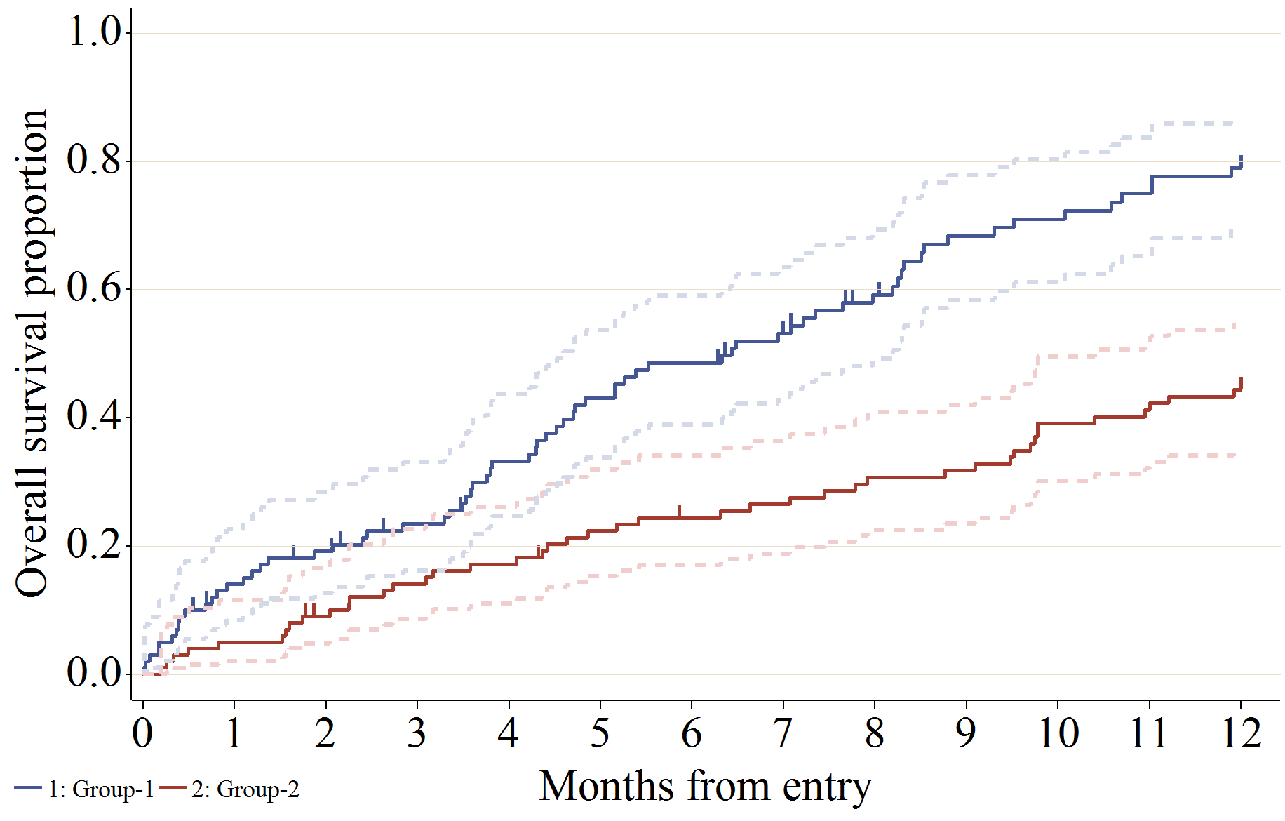
信頼区間 (線を Gplot で描画)、Failure plot (1 - 生存関数の推定値) を描画する場合の設定例です。
  /*****************************************************************/
  /* CI: line, Failure plot */
  data data;
    length strata $20.;
    tc = 12;  /* time to termination */
    h1 = 0.15; n1 = 100;
    h1 = 0.07; n2 = 100;
    array h[*] h1-h1; array n[*] n1-n2;
    do group = 1 to 2;
      do i = 1 to n[group];
        time = rand('exponential') / h[group]; censor = 0;
        /* termination */
        if time > tc then do; time = tc; censor = 1; end;
        /* random censoring */
        if rand('Uniform') > 0.9 then do; censor = 1; end;
        if group = 1 then do; strata = "1: Group-1"; end;
        if group = 2 then do; strata = "2: Group-2"; end;
        output;
      end;
    end;
    label time = "Months after entry";
    keep time censor group strata;
  run;

  %km_data(
  data, time, strata, censor, 1,
  out = graph, anno = anno, afont = "'Times New Roman'",
  failure = 1,
  censEXT  = 1
  );
  goptions reset = all;
  goptions vsize = 12 in hsize = 19 in htitle = 3.5 htext = 3.5;
  filename grafout "&Path.example7.&filetype.";
  goptions device = &filetype. gsfname = grafout gsfmode = replace;
  goptions ftext = "Times New Roman";
  data Graph;
    length vname $10.;
    set Graph;
    var=Sv1; vname='Sv1'; output;
    var=Sv2; vname='Sv2'; output;
    var=SL1; vname='ySL1'; output;
    var=SL2; vname='ySL2'; output;
    var=SU1; vname='ySU1'; output;
    var=SU2; vname='ySU2'; output;
  proc gplot data = graph;
  plot var * time = vname /
    anno = anno autovref cautovref = cxE9DECA
    overlay skipmiss noframe legend = legend1
    haxis = axis1 vaxis = axis2;
  axis1 label = ('Months from entry') major=(w=2 height=0.7) w=2 minor = none
    offset = (2, 7);
  axis2 label = (a=90 'Overall survival proportion') major=(w=2 height=1)
    w=2 minor = none offset = (2, 2) order = (0 to 1 by 0.2);
  legend1 label = none position = (inside)
    mode = share across = 2 origin = (2, 1) value = (h = 2 "1: Group-1" "2: Group-2")
    order = ("Sv1" "Sv2");
  symbol1 i = steplj c="&color1" w = 5;
  symbol2 i = steplj c="&color2" w = 5;
  symbol3 i = steplj c="&scolor1" w = 5 l = 2;
  symbol4 i = steplj c="&scolor2" w = 5 l = 2;
  symbol5 i = steplj c="&scolor1" w = 5 l = 2;
  symbol6 i = steplj c="&scolor2" w = 5 l = 2;
  run; quit;
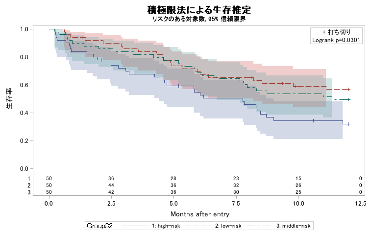
SAS 9.2 ODS Graph との比較
サンプルプログラム [example2.sas] では、まずデフォルトの ODS Graph の出力を行います。
  ods listing gpath = "&Path." style = Statistical sge = on;
  ods graphics on /
    antialias = on border = off scale = on
    imagename = "Lifetest_ods"
    width = 6.33333333 in height = 4 in;
  proc lifetest data = D1 plots=(survival(atrisk=(0 to 12.5 by 2.5) test cl));
    time T * Censor(1);
    strata GroupC2;
  run;
  ods graphics off;
  ods listing close; ods listing;
しかし、普通に用いる場合、軸の名前や線の太さなどを変更する事の方が多いです。
sge 形式 (ods listing sge = on; で出力可能) でグラフを出力し、ODS Graphics Editor
で直接編集してしまう事もできますが、複数のグラフを出力する場合は非効率的です。
そのような場合は Template Procedure を使い、雛形を書き換えてしまうと良いでしょう。
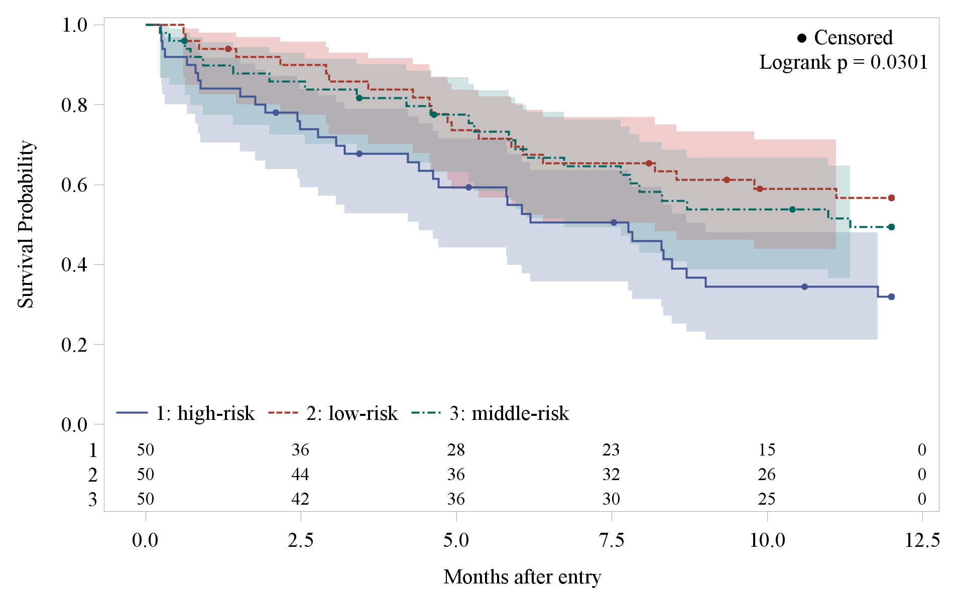
Template Procedure (以下の例は SAS 9.2 のみ対応)
source statement を実行すると、style の定義やグラフの定義が Log ウィンドウに表示されます。
それをコピーして、必要な部分を変更してオリジナルの雛形を作ります。最後に defile statment を用いて定義すると、オリジナルの雛形でグラフを出力できるようになります。
デフォルトの雛形に関しては、以下のスクリプトを実行すると、見る事ができます。
Stat.Lifetest.Graphics.ProductLimitSurvival のようなグラフの名前を調べるには、Results
ウィンドウの各アイコンを右クリックしてプロパティを表示させると、Template の項目の所に書いてあります。
色とフォントを変更する場合は Styles の方を編集します。
  proc template;
    source Styles.Journal2;
    source Stat.Lifetest.Graphics.ProductLimitSurvival;
  run;
  proc template;
  define style Styles.MyStatistical;
  parent = styles.Statistical;
  style GraphFonts /
    'GraphTitleFont'=("Times New Roman",24pt, bold)
    'GraphFootnoteFont'=("Times New Roman",24pt, italic)
    'GraphLabelFont'=("Times New Roman",24pt)
    'GraphValueFont'=("Times New Roman", 24pt)
    'GraphDataFont'=("Times New Roman", 24pt)
    'GraphUnicodeFont'=("<MTsans-serif-unicode>", 24pt)
    'GraphAnnoFont'=("Times New Roman", 24pt);
  end;
グラフの定義はかなり複雑ですので、基本的にヘルプを調べながら更新する事になると思います。
今回は、タイトル・サブタイトルの消去、打ち切り記号の変更、生存曲線の太さを変更、ラベルの変更、凡例の位置変更などを行った雛形を作りました。
  proc template;
  define statgraph Stat.Lifetest.Graphics.ProductLimitSurvival;
    dynamic NStrata xName plotAtRisk plotCensored plotCL plotHW plotEP labelCL labelHW labelEP
        maxTime StratumID classAtRisk plotBand plotTest GroupName yMin Transparency SecondTitle
        TestName pValue;
    BeginGraph;
      if (NSTRATA=1)
        layout overlay / xaxisopts=(shortlabel=XNAME offsetmin=.05 linearopts=(viewmax=MAXTIME))
            yaxisopts=(label="Survival Probability" shortlabel="Survival Probability"
            linearopts=(viewmin=0 viewmax=1 tickvaluelist=(0 .2 .4 .6 .8 1.0)));
          if (PLOTHW=1 AND PLOTEP=0)
            bandplot LimitUpper=HW_UCL LimitLower=HW_LCL x=TIME / modelname="Survival"
                fillattrs=GRAPHCONFIDENCE name="HW" legendlabel=LABELHW;
          endif;
          if (PLOTHW=0 AND PLOTEP=1)
            bandplot LimitUpper=EP_UCL LimitLower=EP_LCL x=TIME / modelname="Survival"
                fillattrs=GRAPHCONFIDENCE name="EP" legendlabel=LABELEP;
          endif;
          if (PLOTHW=1 AND PLOTEP=1)
            bandplot LimitUpper=HW_UCL LimitLower=HW_LCL x=TIME / modelname="Survival"
                fillattrs=GRAPHDATA1 datatransparency=.55 name="HW" legendlabel=LABELHW;
            bandplot LimitUpper=EP_UCL LimitLower=EP_LCL x=TIME / modelname="Survival"
                fillattrs=GRAPHDATA2 datatransparency=.55 name="EP" legendlabel=LABELEP;
          endif;
          if (PLOTCL=1)
            if (PLOTHW=1 OR PLOTEP=1)
              bandplot LimitUpper=SDF_UCL LimitLower=SDF_LCL x=TIME / modelname="Survival"
                  display=(outline) outlineattrs=GRAPHPREDICTIONLIMITS name="CL"
                  legendlabel=LABELCL;
            else
              bandplot LimitUpper=SDF_UCL LimitLower=SDF_LCL x=TIME / modelname="Survival"
                  fillattrs=GRAPHCONFIDENCE name="CL" legendlabel=LABELCL;
            endif;
          endif;
          stepplot y=SURVIVAL x=TIME / name="Survival" rolename=(_tip1=ATRISK _tip2=EVENT)
              tip=(y x Time _tip1 _tip2) legendlabel="Survival Probability"
              LINEATTRS=(thickness=10px);
          if (PLOTCENSORED=1)
            scatterplot y=CENSORED x=TIME / markerattrs=(symbol=CIRCLEFILLED size=8pt)
                name="Censored" legendlabel="Censored";
          endif;
          if (PLOTCL=1 OR PLOTHW=1 OR PLOTEP=1)
            discretelegend "Censored" "CL" "HW" "EP" / location=outside halign=center;
          else
            if (PLOTCENSORED=1)
              discretelegend "Censored" / location=inside autoalign=(topright bottomleft);
            endif;
          endif;
          if (PLOTATRISK=1)
            innermargin / align=bottom;
              blockplot x=TATRISK block=ATRISK / repeatedvalues=true display=(values)
                valuehalign=start valuefitpolicy=truncate labelposition=left
                labelattrs=GRAPHVALUETEXT valueattrs=GRAPHDATATEXT (size=20pt)
                includemissingclass=false;
            endinnermargin;
          endif;
        endlayout;
      else
        layout overlay / xaxisopts=(shortlabel=XNAME offsetmin=.05
            linearopts=(viewmax=MAXTIME)) yaxisopts=(label="Survival Probability"
            shortlabel="Survival Probability"
            linearopts=(viewmin=0 viewmax=1 tickvaluelist=(0 .2 .4 .6 .8 1.0)));
          if (PLOTHW)
            bandplot LimitUpper=HW_UCL LimitLower=HW_LCL x=TIME / group=STRATUM
                index=STRATUMNUM modelname="Survival" datatransparency=Transparency;
          endif;
          if (PLOTEP)
            bandplot LimitUpper=EP_UCL LimitLower=EP_LCL x=TIME / group=STRATUM
                index=STRATUMNUM modelname="Survival" datatransparency=Transparency;
          endif;
          if (PLOTCL)
            if (PLOTBAND)
              bandplot LimitUpper=SDF_UCL LimitLower=SDF_LCL x=TIME / group=STRATUM index=
                STRATUMNUM modelname="Survival" display=(outline);
            else
              bandplot LimitUpper=SDF_UCL LimitLower=SDF_LCL x=TIME / group=STRATUM index=
                STRATUMNUM modelname="Survival" datatransparency=Transparency;
            endif;
          endif;
          stepplot y=SURVIVAL x=TIME / group=STRATUM index=STRATUMNUM name="Survival"
              rolename=(_tip1=ATRISK _tip2=EVENT) tip=(y x Time _tip1 _tip2)
              LINEATTRS=(thickness=3px);
          if (PLOTCENSORED)
            scatterplot y=CENSORED x=TIME / group=STRATUM index=STRATUMNUM
            markerattrs=(symbol=CIRCLEFILLED size=8pt);
          endif;
          if (PLOTATRISK)
            innermargin / align=bottom;
              blockplot x=TATRISK block=ATRISK / class=CLASSATRISK repeatedvalues=true
                display=(label values) valuehalign=start valuefitpolicy=truncate
                labelposition=left labelattrs=GRAPHVALUETEXT
                valueattrs=GRAPHDATATEXT (size=20pt) includemissingclass=false;
            endinnermargin;
          endif;
          DiscreteLegend "Survival" / location=inside HALIGN=LEFT VALIGN=BOTTOM
            border=false;
          if (PLOTCENSORED)
            if (PLOTTEST)
              layout gridded / rows=2 autoalign=(TOPRIGHT BOTTOMLEFT TOP BOTTOM)
                  border=false BackgroundColor=GraphWalls:Color Opaque=true;
                entry "● Censored";
                if (PVALUE < .0001)
                  entry TESTNAME " p " eval (PUT(PVALUE, PVALUE6.4));
                else
                  entry TESTNAME " p = " eval (PUT(PVALUE, PVALUE6.4));
                endif;
              endlayout;
            else
              layout gridded / rows=1 autoalign=(TOPRIGHT BOTTOMLEFT TOP BOTTOM)
                  border=false BackgroundColor=GraphWalls:Color Opaque=true;
                  entry "● Censored";
              endlayout;
            endif;
            else
              if (PLOTTEST)
                layout gridded / rows=1 autoalign=(TOPRIGHT BOTTOMLEFT TOP BOTTOM)
                  border=false BackgroundColor=GraphWalls:Color Opaque=true;
                if (PVALUE < .0001)
                  entry TESTNAME " p " eval (PUT(PVALUE, PVALUE6.4));
                else
                  entry TESTNAME " p = " eval (PUT(PVALUE, PVALUE6.4));
                endif;
                endlayout;
              endif;
            endif;
        endlayout;
      endif;
    EndGraph;
    end;
  run;
設定した雛形を default のものに戻す場合は以下のスクリプトを実行します。
  proc template;
    delete Stat.Lifetest.Graphics.ProductLimitSurvival;
  run;
なお、SAS 9.2 TS2M0 では、どう試しても ODS Graph の出力結果がファイル形式に拠らずラスター画像に変換されてしまった (emf, eps, pdf でもラスターになる)。 ベクトル画像を出力したい場合、現状では ODS Graph は利用できないので、Gplot Procedure を駆使した kmdata マクロが必要になると思われる。
おまけ
また、以下のプログラムを実行すると、style リストを表示する事ができます。
出力サンプル一覧 (pdf)
  /* Print Template List */
  proc template;
   path sashelp.tmplmst;
   list styles;
  run;
SAS 9.2 の ODS Templete 関係で、使えそうなリンクをいくつかリストしておきます。
Templete Procedure を使ってどんどん変更できるので、お気に入りの雛形を作ってしまうと便利です。
Unicode Character (特に記号、ギリシャ文字や数式) への配慮や、ODS HTML などがあるので、Web サービスにそのままリンクさせたりする場合にも便利なようです。
履歴
- 2011/10/19 更新